Face recognition technology is truly usable after deep learning. This is because in previous machine learning techniques, it was difficult to extract appropriate feature values ​​from the picture. contour? colour? eye? With so many faces, and with age, light, shooting angle, color, expression, make-up, accessories, etc., the same person's face photos vary greatly in the pixel level of the photo, with the experience of experts and It is difficult to extract the eigenvalues ​​with high accuracy, and it is naturally impossible to further classify these eigenvalues. The biggest advantage of deep learning is that the training algorithm adjusts the parameter weights by itself and constructs a f(x) function with high accuracy. Given a photo, the feature values ​​can be obtained and then classified.

In this paper, the author tries to explore face recognition technology in popular language. Firstly, it outlines the face recognition technology. Then it discusses the reason why the deep learning is effective and why the gradient decline can train the appropriate weight parameters. Finally, the person based on CNN convolutional neural network is described. Face recognition.

First, an overview of face recognition technology

Face recognition technology is roughly composed of two aspects: face detection and face recognition.

The reason for face detection is not only to detect whether there is a face on the photo, but more importantly, to delete the part of the photo that is not related to the face, otherwise the pixel of the whole photo is passed to the f(x) recognition function. Not available. Face detection does not necessarily use deep learning techniques, because the technical requirements here are relatively low, just need to know if there are any faces and the approximate position of the face in the photo. Generally, we consider using the face detection function of open source libraries such as OpenCV, dlib (the traditional eigenvalue method based on expert experience is less computational and faster), and can also use techniques based on deep learning such as MTCNN (deep in the neural network) When the width is wider, the amount of calculation is larger and slower.)

In the face detection process, we mainly focus on three indicators: detection rate, missed detection rate and false detection rate, among which:

• Detection rate: the proportion of the presence of the face and the detected image in all existing face images; • Missed detection rate: the proportion of images that exist but not detected in all existing face images; • False detection Rate: There is no face but the proportion of the image in which the face exists is detected in all non-existent face images.

Of course, the speed of detection is also important. This article does not further describe face detection.

In the face recognition process, the application scenarios are generally divided into 1:1 and 1:N.

1:1 is to judge whether the two photos are the same person, usually applied to the matching of people's cards, such as whether the ID card and the real-time photo taking are the same person, which is commonly used in various business halls and the registration in the 1:N scene introduced later. Link. The 1:N application scenario is to first perform the registration process, given N inputs including the face photo and its ID identifier, and then perform the identification link, given the face photo as input, and the output is one of the registration links. The ID is either not registered in the photo. It can be seen that from the perspective of probability, the former is relatively simple, and since the document photo usually has an indeterminate time interval with the current photo, the similarity thresholds we usually set are relatively low, so as to obtain a better pass rate. Tolerate a slightly higher rate of false recognition.

The latter 1:N, as N becomes larger, the false recognition rate will increase, and the recognition time will also increase, so the similarity threshold is usually set higher and the pass rate will decrease. Here is a brief explanation of the above nouns: the false recognition rate is the ratio of the photo that is actually A but recognized as B; the pass rate is that the photo is indeed A, but it is possible to identify 4 photos for every 5 photos of A. The pass rate is 80%; the similarity threshold is because the classification of eigenvalues ​​is a probabilistic behavior. Unless the two photos entered are actually the same file, there is a similarity between any two photos. After the similarity threshold, only the similarity of two photos exceeds the threshold, it is considered to be the same person. Therefore, it is meaningless to simply evaluate the accuracy of a face recognition algorithm. What we need to clarify most is the pass rate when the false recognition rate is less than a certain value (for example, 0.1%). Regardless of 1:1 or 1:N, the underlying technology is the same, but the difficulty is different.

It is the most difficult to take out face feature values, so how does deep learning take feature values?

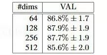
Suppose that the face photo we give is 100*100 pixels. Since each pixel has three channels of RGB, each pixel channel is represented by a byte in the range of 0-255, there are three matrixes of 100*100. Ten thousand bytes are used as input data. Deep learning actually generates an approximation function that converts the above input values ​​into feature values ​​that can be used as feature classifications. So, can the feature value be a number? Of course not, a number (or scalar) is not able to effectively represent the feature. Usually we use a vector of multiple values ​​to represent the eigenvalue, and the dimension of the vector is the number of values ​​in it. The dimension of the feature vector is not as large as possible. The test results of Google's FaceNet project (see https://arxiv.org/abs/1503.03832) show that the feature vector of 128 values ​​is the best, as shown below. :

So, now the question translates into how to convert a 3*100*100 matrix into a 128-dimensional vector, and this vector can accurately distinguish different faces?

Assuming the photo is x, the eigenvalue is y, which means that there is a function f(x)=y that perfectly finds the face feature value of the photo. Now we have an f*(x) approximation function, in which it has a parameter w (or weight w) that can be set, for example, written as f*(x;w). If there is a training set x and its id identifier y, set the initial parameters. After p1, then each time f*(x;w) gets y` compared with the actual mark y, if it is correct, it passes, if it is wrong, the parameter w is adjusted appropriately. If the parameter w can be correctly adjusted, f*(x ;w) will be close enough to the ideal f(x) function, and we obtain a f*(x;w) function with a sufficiently high probability of accuracy. This process is called training under supervised learning. The process of calculating the value of f*(x;w) is a normal function operation, which is called forward operation. When the y is compared with the actual identification id value y in the training process, the process of adjusting the parameter p is reversed. Come over, called backpropagation.

Since the x-input we pass is a photo after all, the photo has both quality problems that are not easy to measure due to focus, light, angle, etc., as well as the number of pixels in itself. If x itself contains too little data, ie the picture is very unclear, such as a 28*28 pixel photo, then no one can tell exactly who it is. It can be imagined that the more the number of pixels is, the more accurate the recognition is, but the more the number of pixels, the greater the computation, transmission, and storage consumption. We need to find the appropriate threshold based on the basis. The following picture is the result of the FaceNet paper. Although it is only a word, Google's rigorous attitude makes the data very valuable.

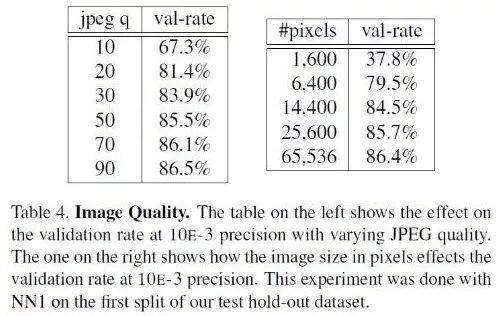
As can be seen from the figure, in addition to the other qualities of the photo, the number of pixels must be at least 100*100 (pure face part) to ensure a relatively high recognition rate.

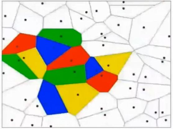
Second, the principle of deep learning technology

What kind of function f(x) should be designed to be converted into eigenvalues ​​from the pixel value matrix transformed by the clear face? The answer to this question depends on the classification problem. That is, let's not talk about feature values ​​first. How do you first correctly classify photo collections by people? Here is a talk about machine learning. Machine learning believes that algorithms can be well generalized from a limited set of training sets. Therefore, we first find a limited training set, design the initial function f(x; w), and have quantified the training set x->y. If the data x is low-dimensional and simple, such as only two-dimensional, the classification is simple, as shown in the following figure:

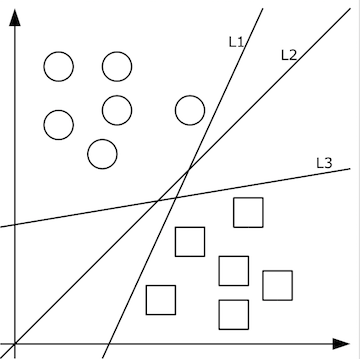
The two-dimensional data x in the above figure has only two categories y, square and circular. It is very good. The classification function we need to learn can represent the classification line with the simplest f(x, y)=ax+by+c. . For example, if f(x, y) is greater than 0, it means a circle, and when it is less than 0, it means a square.

Given the random number as the initial value of a, c, b, we continuously optimize the parameters a, b, c through the training data, and gradually train the inappropriate L1, L3 and other classification functions into L2, so that L2 faces the pan The test data is likely to get better results. However, if there are multiple categories, multiple classification lines are required to separate them, as shown in the following figure:

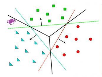
This is actually equivalent to the result of multiple classification functions executing with &&, or || operations. At this time, it is also possible to use a classification function such as f1>0 && f2<0 && f3>0, but if it is more complicated, for example, the characteristics of itself are not obvious and are not gathered together, this way of finding features cannot be played. As shown in the figure below, different colors indicate different classifications, and the training data at this time is completely non-linearly separable:

At this time, we can solve it by multi-level function nesting, such as f(x)=f1(f2(x)), so that the f2 function can be several lines, and the f1 function can pass different weights w and excitation. The function completes with &&, or || and so on. There are only two layers of functions. If the number of function nesting levels is more, it can express complex classification methods, which is very helpful for high-dimensional data. For example, our photos are undoubtedly such input. The so-called excitation function is to convert the very large value range calculated by the function f into a smaller value range such as [0, 1], which allows the multi-layer function to continuously forward and classify.

The forward operation simply passes the input to the f1(x, w1) function, the calculated value is passed to the f2(y1, w2) function, and so on, and the final classification value is very simple. However, because the initial w weight does not really make much sense, the resulting classification value f*(x) is definitely wrong. We know the correct value y on the training set, so in fact we actually want yf*(x The value of ) is the smallest, so the classification is more accurate. This actually becomes a problem of finding the minimum. Of course, yf*(x) is just a sign. In fact, the f*(x) we get is only the probability of falling on each classification. The process of comparing this probability with the real classification to get the minimum value is called the loss function. Its value is loss, and our goal is to minimize the loss of the loss function. In the face recognition scene, softmax is a better loss function, let's take a look at how it is used.

For example, we have training dataset photos corresponding to cat, dog, ship three categories, an input photo through the function f (x) = x * W + b, forward calculation to get the score of the three categories of the photo . At this point, this function is called the score function, as shown in the following figure, assuming that the input image on the left is a 4-dimensional vector [56, 231, 24, 2], and the W weight is a 4 * 3 matrix, then multiply After adding the vector [1.1, 3.2, -1.2], you can get the scores in the cat, dog, and ship categories:

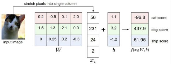
As can be seen from the example above, although the input photo is a cat, the score on the score is 437.9, but what is the height of the cat and the boat? Hard to measure! If we convert the score value to a percentage probability of 0-100, this is convenient to measure. Here we can use the sigmoid function, as shown below:

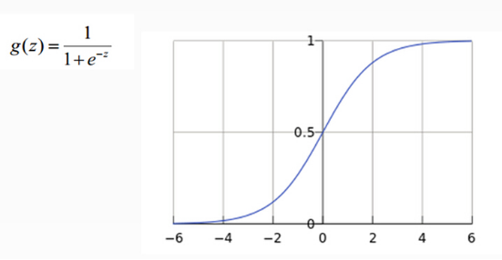
From the above formula and graph, sigmoid can convert any real number to a number between 0-1 as a probability. However, the sigmoid probability is not normalized, which means that we need to ensure that the sum of the probabilities of the input photos in all categories is 1, so we also need to do the following processing on the score value in softmax mode:

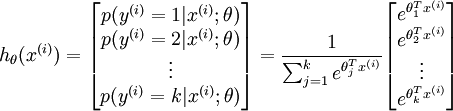
This gives x the probability of x under each category given x. Assuming that the scores of the three categories are 3, 1, and -3, respectively, the probability obtained by the above formula is [0.88, 0.12, 0], and the calculation process is as follows:

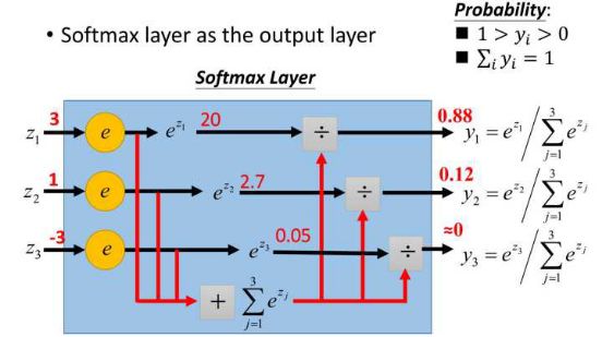
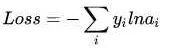
However, the probability of x is actually the first class, such as [1,0,0], and the probability (or can be called likelihood) that is obtained now is [0.88, 0.12, 0]. So how big is the gap between them? This gap is the loss value loss. How to get the loss value? In softmax we use the mutual entropy loss function to calculate the least amount (convenient to derive), as shown below:

Where i is the correct classification, for example the loss value in the above example is -ln0.88. So after we have the loss function f(x), how can we adjust the x to minimize the loss value of the function? This involves differential derivatives.

Third, the gradient decline

The gradient descent is to quickly adjust the weight w such that the value of the loss function f(x; w) is the smallest. Because the value of the loss function has the least loss, it means that the score on the training set is the closest to the correct classification value!

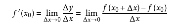
The derivative is the rate of change of the function at a certain point. For example, driving from point A to point B, the average speed can be calculated by distance and time, but what is the instantaneous speed of point C? If x is used to represent time and f(x) is the distance from the point A, then the instantaneous speed at x0 can be converted to: a small time from x0, for example 1 second, then this second The average speed is the distance traveled by this second divided by 1 second, which is (f(1+x0)-f(x0))/1. If we are not using 1 second but 1 microsecond, then the average speed in 1 microsecond is necessarily closer to the instantaneous speed at x0. Thus, by the time period t tending to zero, we get the instantaneous velocity at x0. This instantaneous velocity is the rate of change of the function f over x0, and the rate of change over all x constitutes the derivative of the function f(x), called f`(x). which is:

From a geometric point of view, the rate of change becomes a slope, which makes it easier to understand how to find the minimum value of a function. For example, in the figure below, the function y=f(x) is represented by a bold black line, and its rate of change at point P0 is the slope of the tangent red line:

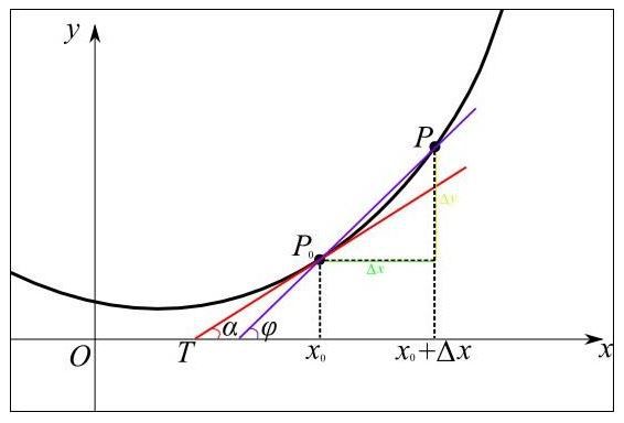
It can be seen visually that when the value of the slope is positive, move x to the left to become smaller, and the value of f(x) will be smaller; when the value of the slope is negative, move x to the right to become larger. Some, the value of f(x) will be smaller, as shown in the following figure:

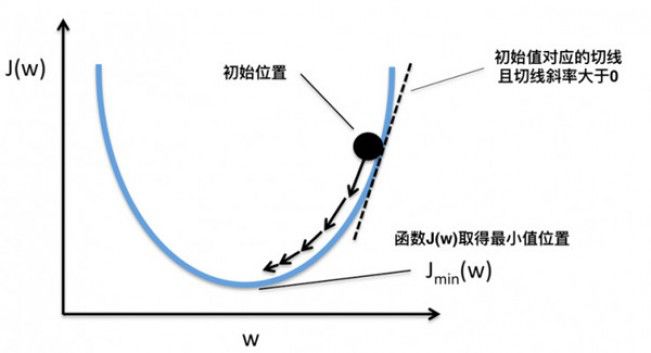
Thus, when the slope is 0, we actually get the function f at which the minimum value can be obtained. So, move x to the left or right, how much does it move? If you move more, you may have moved it. If you move it very little, you may have to move it for a long time to find the minimum point. There is also a problem. If the f(x) operation function has multiple local minimum points and global minimum points, if the x shift is very small, it may cause only a local minimum point that is not small enough to be found by the derivative. As shown below:

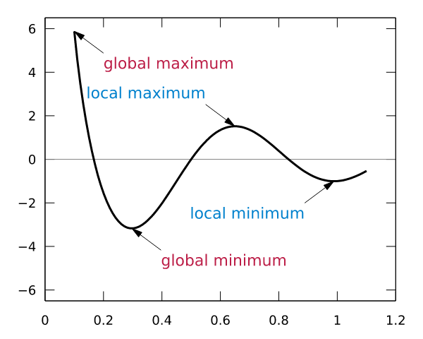
Blue is the local minimum point and red is the global minimum point. So how much x moves is a problem, and each move step size is too large or too small may result in the global minimum point not being found. In addition to the derivative slope, we also need a hyperparameter to control its moving speed. This hyperparameter is called the learning rate. Because it is difficult to optimize, it usually needs to be set manually and cannot be adjusted automatically. Considering that training time is also a cost, we usually set the learning rate to be larger in the initial training phase, and the learning rate is set to be smaller.

So is the step size of each move related to the value of the derivative? This is natural, the positive and negative values ​​of the derivative determine the direction of movement, and the absolute value of the derivative determines whether the slope is steep. The steeper the move, the larger the step size should be. Therefore, the step size is determined by the learning rate and the derivative. Like this function, λ is the learning rate, and ∂F(ωj) / ∂ωj is the derivative at the point ωj.

Ωj = ωj – λ ∂F(ωj) / ∂ωj

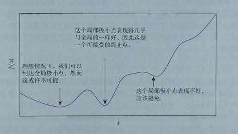
According to the derivative, the method of how the loss function f should move at the point x0 to make f reach the minimum value is called gradient descent. The gradient is also the derivative. In the direction of the negative gradient, the moving step is controlled according to the gradient value, and the minimum value can be quickly reached. Of course, in fact we may not be able to find the minimum point, especially if there are multiple minimum points in itself, but if the value itself is small enough, we can also accept it, as shown below:

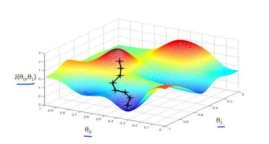
Above we look at the gradient drop in one-dimensional data, but our photo is multidimensional data. How do we find the derivative? How is the gradient falling? At this point we need to use the concept of partial derivatives. In fact, it is very similar to the derivative. Since x is a multidimensional vector, then we assume that when calculating the derivative of Xi, the other values ​​on x are unchanged, which is the partial derivative of Xi. At this time, the gradient descent method is applied as shown in the following figure. θ is two-dimensional. We can find the derivative of θ0 and θ1 respectively, and then move the corresponding step from both θ0 and θ1 to find the lowest point, as shown in the following figure. Show:

As mentioned above, according to the limited training set, to adapt to the infinite test set, of course, the larger the training set capacity, the better the effect. However, if the training set is large, then the amount of gradient descent calculation based on all the data is too large. At this point, we choose to take only a small part of the total training set at a time (how much, depending on the amount of memory and calculations), perform gradient descent, continuous iteration, and quickly reduce the gradient as experienced. This is the random gradient drop.

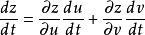
The gradient descent method above can only adjust the w weight of the f function, and we have said that the actual multi-layer function is put together, for example, f1(f2(x;w2);w1), then how to find each What is the derivative of the layer function input? This is also how the so-called backpropagation continues to be reversed. This is to mention the chain rule. The essence is that the original y to x can be achieved by introducing the intermediate variable z, as shown in the following figure:

Thus, the derivative of y versus x is equivalent to the derivative of y versus z multiplied by the partial derivative of z versus x. When the input is multidimensional, there is the following formula:

In this way, we can get the derivative of each layer of function, so that we can get the step size of the weight of each layer function should be adjusted, optimize the weight parameters.

Since the derivative of the function is very large, for example, the network such as resnet has reached 100 multi-layer functions, so to distinguish the traditional machine learning, we call it deep learning.

Deep learning is only inspired by neuroscience, so it is called neural network, but it is essentially the multi-function forward operation mentioned above to get the classification value. After training, the loss function is minimized according to the actual label classification, and then it is reduced according to the random gradient. Method to optimize the weight parameters of each layer function. Face recognition is also such a process. Above we have initially completed the parameter adjustment of the multi-layer function, but how should the function itself be designed?

Fourth, face recognition based on CNN convolutional neural network

Let's start with a fully connected network. Google's TensorFlow playground can intuitively experience the power of a fully connected neural network. This is the playground's website: http://playground.tensorflow.org/, you can do neural network training in the browser, and visualize the process and results. . As shown below:

This neural network playground has a total of 1000 training points and 1000 test points for dividing blue and yellow points into 4 different patterns. There are 4 different patterns to choose from at DATA.

The input layer of the entire network is FEATURES (features of the problem to be solved). For example, x1 and x2 represent vertical or horizontal segmentation to divide blue and yellow dots, which is the easiest way to understand the two points. The other five are actually not easy to think of. This is what the traditional expert system only needs. In fact, this playground is for demonstration. 1. A good neural network can only use the input layer FEATURES such as x1 and x2. Perfect implementation; 2, even if there are many input features, we don't know who has the highest weight, but a good neural network will solve this problem.

HIDDEN LAYERS can set the number of layers at will, and each hidden layer can set the number of neurons. In fact, the neural network is not in the case of sufficient computing power, the more layers the better or the more neurons per layer, the better. A good neural network architecture model is hard to find. Later in this article we will focus on several CNN classic network models. However, in this example, more hidden layers and neurons can be better divided.

Epoch is the number of rounds of training. The loss value in the red box is the most important indicator to measure the training result. If the loss value is always decreasing, for example, it can be as low as 0.01, which means that the result of this network training is good. Loss may also drop for a while and then suddenly rise, this is a bad network, you can try it. The learning rate will be set higher initially, and will be lowered after training. Activation is an incentive function, and currently CNN is using the Relu function.

After learning about the neural network, now we are back to face recognition. Each layer of neurons is an f function, and the upper four layers of the network are f1 (f2(f3(f4(x))))). However, as mentioned above, there are too many pixels in a photo, and every two neurons between any two layers in a fully connected network need to have one calculation. As mentioned earlier, complex classification relies on the joint operation of many layer functions to achieve the goal. Many of the current networks are more than 100 layers. If each layer has 3*100*100 neurons, you can imagine how much calculation! The CNN convolutional neural network came into being, which can greatly reduce the amount of computation while preserving the power of a fully connected network.

CNN believes that it is possible to perform a full join operation on only one rectangular window of the entire picture (which can be called a convolution kernel). After sliding the window and traversing the entire picture with the same weight parameter w, the input of the next layer can be obtained, as shown in the following figure. Shown as follows:

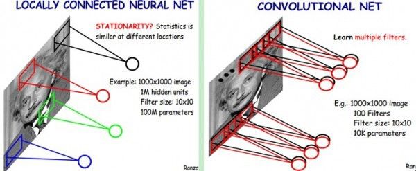
The CNN considers that the weight parameters in the same layer can be shared because each different region of the same picture has a certain similarity. In this way, the original full connection calculation is too large to solve the problem, as shown in the following figure:

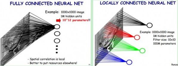
Combining the previous function forward operations and matrices, we take a dynamic picture to visually look at the forward operation process:

Here the convolution kernel size and the moving stride and the output depth determine the size of the next layer of the network. At the same time, when the kernel size and the stride step size cause the upper layer matrix to be not large enough, padding is required to fill 0 (the gray of the above figure is 0). This is called a convolution operation. Such a layer of neurons is called a convolutional layer. In the above figure, W0 and W1 indicate a depth of 2.

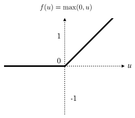
The CNN convolutional network usually adds an excitation layer after each layer of the convolutional layer. The excitation layer is a function that converts the value of the output of the convolutional layer into a nonlinear value in a non-linear manner, and constrains while maintaining the size relationship. The range of values ​​allows the entire network to be trained. In face recognition, the Relu function is usually used as the excitation layer, and the Relu function is max(0, x), as shown below:

It can be seen that the amount of calculation of Relu is actually very small!

There is also a pooling layer in CNN. When the amount of data outputted by a layer is too large, the data can be dimensionally reduced by the pooling layer, and the amount of data can be reduced while maintaining the feature. For example, the following 4*4 matrix passes. Take the maximum value to reduce the dimension to the 2*2 matrix:

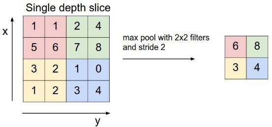
In the above figure, the maximum number is filtered by each color block to reduce the amount of calculation data.

Usually the last layer of the network is a fully connected layer, so the general CNN network structure is as follows:

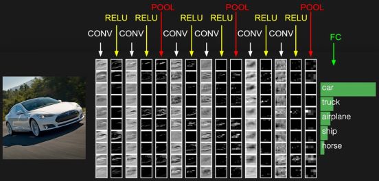
CONV is the convolutional layer, which carries the RELU layer after each CONV. This is just a schematic diagram, and the actual network is much more complicated. At present, the open source Google FaceNet uses the resnet v1 network for face recognition. For the resnet network, please refer to the paper https://arxiv.org/abs/1602.07261. The complete network is more complicated, it is not listed here, you can also view it. Based on the Python code implemented by TensorFlow https://github.com/davidsandberg/facenet/blob/master/src/models/inception_resnet_v1.py, note that slim.conv2d contains the Relu stimulus layer.

The above is just a general CNN network. Since the face recognition application is not directly classified, but has a registration phase, the feature value of the photo needs to be taken out. If the data before softmax classification is directly used as the feature value, the effect is very bad. For example, the following figure directly converts the output of the fully connected layer into a two-dimensional vector, and the visual representation of the classification is represented by color on the two-dimensional plane:

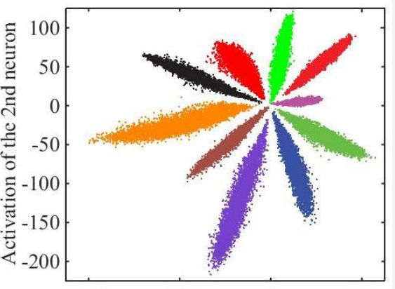
The visible effect is not good, the sample distance in the middle is too close. After processing by the centor loss method, the distance between the feature values ​​can be expanded, as shown in the following figure:

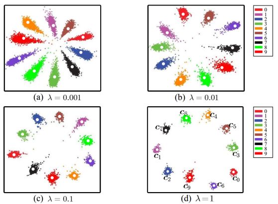
The feature value thus taken out will be much better.

When actually training the resnet v1 network, you first need to pay attention to the quality of the training set photos, and resize the face photos of different sizes to the size received by the first layer of the resnet1 network. In addition to the above mentioned learning rate and the number of batchsize pictures in the random gradient drop, you need to set the epochsize correctly, because each round of epoch should completely traverse the training set, and the batchsize is limited by the hardware conditions. Not constant, but the training set may have been getting bigger, so keep epochsize*batchsize close to all training sets. During the training process, it is necessary to pay close attention to whether the loss value is converging, and the learning rate can be appropriately adjusted.

Finally, the only standard for the evaluation of face recognition is LFW (Labeled Faces in the Wild), which contains 12,000 photos of about 6,000 different people, and many algorithms use it to evaluate the accuracy. But it has two problems, one is that the data set is not big enough, and the other is that the data set scene often does not match the real application scenario. So if an algorithm says how accurate its LFW is, it doesn't reflect its true availability.

ZGAR Classic 1.0

AURORA SERIES DISPOSABLE VAPE PEN

Zgar 2021's latest electronic cigarette Aurora series uses high-tech temperature control, food grade disposable pod device and high-quality material.Compared with the old model, The smoke of the Aurora series is more delicate and the taste is more realistic ,bigger battery capacity and longer battery life. And it's smaller and more exquisite. A new design of gradient our disposable vape is impressive. We equipped with breathing lights in the vape pen and pod, you will become the most eye-catching person in the party with our atomizer device vape.

The 2021 Aurora series has upgraded the magnetic suction connection, plug and use. We also upgrade to type-C interface for charging faster. We have developed various flavors for Aurora series, Aurora E-cigarette Cartridge is loved by the majority of consumers for its gorgeous and changeable color changes, especially at night or in the dark. Up to 10 flavors provide consumers with more choices. What's more, a set of talking packaging is specially designed for it, which makes it more interesting in all kinds of scenes. Our vape pen and pod are matched with all the brands on the market. You can use other brand's vape pen with our vape pod. Aurora series, the first choice for professional users!

We offer low price, high quality Disposable E-Cigarette Vape Pen,Electronic Cigarettes Empty Vape Pen, E-cigarette Cartridge,Disposable Vape,E-cigarette Accessories,Disposable Vape Pen,Disposable Pod device,Vape Pods,OEM vape pen,OEM electronic cigarette to all over the world.

ZGAR Classic 1.0 Disposable Pod Vape,ZGAR Classic 1.0 Disposable Vape Pen,ZGAR Classic 1.0,ZGAR Classic 1.0 Electronic Cigarette,ZGAR Classic 1.0 OEM vape pen,ZGAR Classic 1.0 OEM electronic cigarette.

Zgar International (M) SDN BHD , https://www.szvape-pen.com