
Classification problems are common problems in machine learning applications, and two classification problems are typical, such as the identification of spam. This paper is based on the bank marketing dataset in the UCI machine learning database. From the exploration of datasets, data preprocessing and feature engineering, to the evaluation and selection of learning models, the paper outlines the general process of solving classification problems. The paper contains some common problems, such as the processing of missing values, how to encode non-numeric attributes, how to use oversampling and undersampling to solve the problem of imbalance between positive and negative samples in classification problems.
1. Dataset selection and problem definition
This experiment selects the Bank Marketing Data Set (http://archive.ics.uci.edu/ml/datasets/Bank+Marketing) in the UCI Machine Learning Library. These data relate to direct marketing activities of Portuguese banking institutions. These direct marketing campaigns are based on the phone. In general, the banking agency's customer service staff needs to contact the customer at least once to find out if the customer will subscribe to the bank's products (time deposits). Therefore, the task corresponding to the data set is a classification task, and the classification target is to predict whether the customer is (yes) or not (no) subscribes to the time deposit (variable y).
The data set contains four csv files:
1) bank-additional-full.csv: contains all the samples (41188) and all feature inputs (20), sorted by time (from May 2008 to September 2010);
2) bank-additional.csv: randomly select 10% of the samples from 1) (4119);
3) bank-full.csv: Contains all the samples (41188) and 17 feature inputs, sorted by time. (The data set is an older version with fewer feature inputs);
4) bank.csv: randomly select 10% of the 4119 samples from 3).
Small data sets (bank-additional.csv and bank.csv) are provided to be able to quickly test some computationally expensive machine learning algorithms (such as SVM). This experiment will select a newer data set, 1) and 2) containing 20 feature quantities.
2. Know the data
2.1 data set input variables and output variables
The input variables of the data set are 20 feature quantities, which are divided into numeric variables and categorical variables. See the dataset website at http://archive.ics.uci.edu/ml/datasets/Bank+Marketing for a detailed description.
The output variable is y, that is, whether the customer has subscribed to a time deposit (binary: "yes", "no").
2.2 Raw data analysis
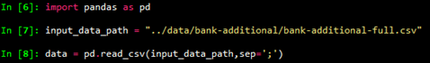
Load the data first,
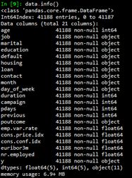
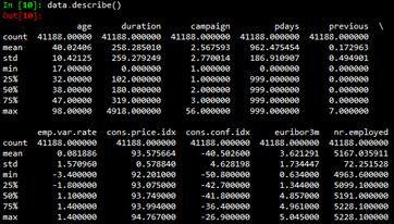
Then use the info() function and the describe() function to see the basic information of the data set.
3. Data Preprocessing and Feature Engineering
3.1 Missing value processing
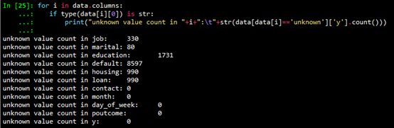
As can be seen from the basic information of the data set given in Section 2.2, the numeric variables (int64 and float64) are not missing. Non-numeric variables may have unknown values. Use the following code to see the number of unknown values ​​for character variables.
Missing value processing usually has the following methods:
For variables with a small number of unknown values, including job and marital, delete these variables as rows with unknown values ​​(unknown);
If the variable is expected to have little effect on the learning model, you can assign a mode to the unknown value. Here, the variables are considered to have a greater impact on the learning model. This method is not adopted.
You can use the complete row of data as a training set to predict missing values, and the missing values ​​of the variables housing, loan, education, and default take this approach. Since the sklearn model can only process numeric variables, you need to first quantify the categorical variables and then make predictions. This experiment uses random forests to predict missing values. The code is as follows:
Def fill_unknown(data, bin_attrs, cate_attrs, numeric_attrs):
#fill_attrs = ['education', 'default', 'housing', 'loan']
Fill_attrs = []
For i in bin_attrs+cate_attrs:
If data[data[i] == 'unknown']['y'].count() < 500:
# delete col containing unknown
Data = data[data[i] != 'unknown']
Else:
Fill_attrs.append(i)
Data = encode_cate_attrs(data, cate_attrs)
Data = encode_bin_attrs(data, bin_attrs)
Data = trans_num_attrs(data, numeric_attrs)
Data['y'] = data['y'].map({'no': 0, 'yes': 1}).astype(int)
For i in fill_attrs:
Test_data = data[data[i] == 'unknown']
testX = test_data.drop(fill_attrs, axis=1)
Train_data = data[data[i] != 'unknown']
trainY = train_data[i]
trainX = train_data.drop(fill_attrs, axis=1)
Test_data[i] = train_predict_unknown(trainX, trainY, testX)
Data = pd.concat([train_data, test_data])
Return data
3.2 Classification variable numericalization
In order to enable categorical variables to participate in model calculations, we need to quantify categorical variables, that is, coding. The categorical variables can be further divided into two categorical variables, ordered categorical variables and unordered categorical variables. There are also differences in the way in which different types of categorical variables are encoded.
3.2.1 Two-class variable coding
According to the input variable description above, the variables default, housing, and loan can be considered as two-category variables, which are encoded by 0,1. code show as below:
Def encode_bin_attrs(data, bin_attrs):
For i in bin_attrs:
Data.loc[data[i] == 'no', i] = 0
Data.loc[data[i] == 'yes', i] = 1
Return data
3.2.2 Ordered categorical variable coding
According to the input variable description above, the variable education can be considered as an ordered categorical variable, and the size order is "illiterate", "basic.4y", "basic.6y", "basic.9y", "high.school", "professional.course", "university.degree", variable influences are encoded as 1, 2, 3, ..., from small to large. code show as below:
Def encode_edu_attrs(data):
Values ​​= ["illiterate", "basic.4y", "basic.6y", "basic.9y",
"high.school", "professional.course", "university.degree"]
Levels = range(1,len(values)+1)
Dict_levels = dict(zip(values, levels))
For v in values:
Data.loc[data['education'] == v, 'education'] = dict_levels[v]
Return data
3.2.3 Unordered categorical variable coding
According to the input variable description above, the variables job, marital, contact, month, day_of_week can be considered as unordered categorical variables. It should be noted that although the variables month and day_of_week are ordered from a time perspective, they are unordered for the target variable. For unordered categorical variables, they can be encoded using dummy variables. In general, n categories need to set n-1 dummy variables. For example, the variable marital is divided into divorced, married, single, encoded using two dummy variables V1 and V2.
| Marital | V1 | V2 |
| Divorced | 0 | 0 |
| Married | 1 | 0 |
| Single | 0 | 1 |
Python's pandas package provides functions for generating dummy variables, so the code looks like this:
Def encode_cate_attrs(data, cate_attrs):
Data = encode_edu_attrs(data)
Cate_attrs.remove('education')
For i in cate_attrs:
Dummies_df = pd.get_dummies(data[i])
Dummies_df = dummies_df.rename(columns=lambda x: i+'_'+str(x))
Data = pd.concat([data,dummies_df], axis=1)
Data = data.drop(i, axis=1)
Return data
3.3 Numerical feature preprocessing
3.3.1 Continuous feature discretization
One of the benefits of discretizing continuous features is that they can effectively overcome hidden defects in the data: making the model results more stable. For example, extreme values ​​in the data are an important factor influencing the effects of the model. Extreme values ​​cause the model parameters to be too high or too low, or cause the model to be "confusing" by false phenomena, and learn the relationship that does not exist as an important model. Discretization, especially equidistant dispersion, can effectively attenuate the effects of extreme values ​​and outliers.
By observing the statistics of the original data set in Section 2.2, we can see that the maximum value of the variable duration is 4918, and the 75% quantile is 319, which is much smaller than the maximum value, and the standard deviation of the variable is 259, which is relatively large. . Therefore, the variable duration is discretized. Specifically, the pandas.qcut() function is used to discretize continuous data, which uses quantile to divide the data (bining: bining), and can obtain bins of substantially equal size, expressed in intervals. Then use the pandas.factorize() function to convert the range to a numeric value.
Data[bining_attr] = pd.qcut(data[bining_attr], bining_num)
Data[bining_attr] = pd.factorize(data[bining_attr])[0]+1
3.3.3 Normalization
Since different variables often use different units of measure, they differ greatly in numerical value, making it easier for distance-based learning models to be more susceptible to larger values. Data normalization is the compression of data into a range, so that the unit impact of all variables is consistent.
For i in numeric_attrs:
Scaler = preprocessing.StandardScaler()
Data[i] = scaler.fit_transform(data[i])
3.3.4 Persistence of preprocessed data
Due to the need to train the model to predict unknown values, the time cost of the preprocessing process is relatively large. Therefore, the pre-processed data is persisted and saved to a file, and the subsequent learning model directly reads the file data for training prediction without further pre-processing.
Def preprocess_data():
Input_data_path = "../data/bank-additional/bank-additional-full.csv"
Processed_data_path = '../processed_data/bank-additional-full.csv'
Print("Loading data...")
Data = pd.read_csv(input_data_path, sep=';')
Print("Preprocessing data...")
Numeric_attrs = ['age', 'duration', 'campaign', 'pdays', 'previous',
'emp.var.rate', 'cons.price.idx', 'cons.conf.idx',
'euribor3m', 'nr.employed',]
Bin_attrs = ['default', 'housing', 'loan']
Cate_attrs = ['poutcome', 'education', 'job', 'marital',
'contact', 'month', 'day_of_week']
Data = shuffle(data)
Data = fill_unknown(data, bin_attrs, cate_attrs, numeric_attrs)
Data.to_csv(processed_data_path, index=False)
It should be noted that since the original data is ordered (in time order), after reading the original data, it needs to be randomly scrambled to become an unordered data set. This uses the shuffle() function in the sklearn.utils package to mess up.
In some cases, the raw data dimensions are very high. The higher the dimension, the more sparse the distribution of data in each feature dimension. This is basically a catastrophic (dimension disaster) for machine learning algorithms. When we have no way to pick out valid features, we need to use algorithms such as PCA to reduce the data dimension so that the data can be used in statistical learning algorithms. However, if you can pick out fewer and more refined features, then the PCA and other dimensionality reduction algorithms are not necessary. In this experiment, the characteristics of the data set have been representative and not too much, so there should be no need to reduce the dimension (experimental proof that dimension reduction does not help). For an introduction to dimension reduction, please refer to this blog (http://).
In short, data preprocessing is very important for training machine learning algorithms, which is called "garbage in, garbage out".
4. Model training and evaluation
4.1 Dividing the data set
First, the processed data set needs to be divided into three parts, which are a train set, a cross validation set, and a test set. (See also the evaluation and selection of the blog learning model). The training set is used to train the model. The cross-check set is used to select the model, including selecting different models or different parameters of the same model, that is, selecting the model with the best test results on the cross-check set. The test set is used to detect the quality of the final selected optimal model. Usually, it can be divided according to the ratio of 6:2:2, the code is as follows:
Def split_data(data):
Data_len = data['y'].count()
Split1 = int(data_len*0.6)
Split2 = int(data_len*0.8)
Train_data = data[:split1]
Cv_data = data[split1:split2]
Test_data = data[split2:]
Return train_data, cv_data, test_data
4.2 Training Set Resampling
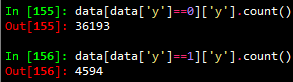
A simple statistic of the imported data set as follows can be found that the number of positive samples (y = 1) is much smaller than the number of negative samples (y = 0), which is approximately equal to 1/8 of the number of negative samples.
In the classification model, this data imbalance problem makes the learning model tend to divide the sample into a majority class, but we are often more concerned about the prediction of a few classes. In this classification problem, the classification target is to predict whether the customer is (yes: 1) no (no: 0) subscribes to the time deposit (variable y). Obviously, we are more concerned about which customers subscribe to time deposits. To mitigate the adverse effects of data imbalances, there are two simpler methods at the data level: oversampling and undersampling.
Oversampling: The most common method of sampling unbalanced data. The basic idea is to eliminate or reduce data imbalance by changing the distribution of training data. The oversampling method improves the classification performance of a few classes by adding a few class samples. The simplest method is to simply copy a few class samples. The disadvantage is that it may lead to overfitting, without adding any new information to a few classes, and the generalization ability is weak. The improved oversampling method involves adding random Gaussian noise or generating new synthetic samples to a few classes.
Undersampling: Undersampling method improves the classification performance of a few classes by reducing the majority of samples. The easiest way is to reduce the size of most classes by randomly removing some majority samples. The disadvantage is that some important information of most classes will be lost. Can not make full use of existing information.
In this experiment, a new sample was added for sampling using the Smoke algorithm [Chawla et al., 2002]; under-sampling was performed by randomly removing some of the majority samples. The basic idea of ​​the Smote algorithm is to calculate the distance from all samples in a few classes to the distances of all samples in a few sample sets for each sample x in a few classes, and get its k-nearest neighbors. Then, a sampling ratio is set according to the sample imbalance ratio to determine the sampling magnification N. For each minority sample x, several samples are randomly selected from their k nearest neighbors to construct a new sample. For the data of this experiment, in order to prevent the newly generated data from being too noisy, only the numerical variables are newly generated in the new sample, and other variables are consistent with the original samples. The resampled code is as follows:
Def resample_train_data(train_data, n, frac):
Numeric_attrs = ['age', 'duration', 'campaign', 'pdays', 'previous',
'emp.var.rate', 'cons.price.idx', 'cons.conf.idx',
'euribor3m', 'nr.employed',]
#numeric_attrs = train_data.drop('y',axis=1).columns
Pos_train_data_original = train_data[train_data['y'] == 1]
Pos_train_data = train_data[train_data['y'] == 1]
New_count = n * pos_train_data['y'].count()
Neg_train_data = train_data[train_data['y'] == 0].sample(frac=frac)
Train_list = []
If n != 0:
Pos_train_X = pos_train_data[numeric_attrs]
pos_train_X2 = pd.concat([pos_train_data.drop(numeric_attrs, axis=1)] * n)
Pos_train_X2.index = range(new_count)
s = smote.Smote(pos_train_X.values, N=n, k=3)
pos_train_X = s.over_sampling()
pos_train_X = pd.DataFrame(pos_train_X, columns=numeric_attrs,
Index=range(new_count))
Pos_train_data = pd.concat([pos_train_X, pos_train_X2], axis=1)
Pos_train_data = pd.DataFrame(pos_train_data, columns=pos_train_data_original.columns)
Train_list = [pos_train_data, neg_train_data, pos_train_data_original]
Else:
Train_list = [neg_train_data, pos_train_data_original]
Print("Size of positive train data: {} * {}".format(pos_train_data_original['y'].count(), n+1))
Print("Size of negative train data: {} * {}".format(neg_train_data['y'].count(), frac))
Train_data = pd.concat(train_list, axis=0)
Return shuffle(train_data)
4.3 Model training and evaluation
Common classification models include perceptron, SVM, naive Bayes, decision tree, logistic regression, random forest, and so on. In this experiment, logistic regression and random forest were selected for training on the training set. The evaluation was performed on the cross-test set. The performance of the random forest was better. Therefore, the random forest model was selected to test on the test set.
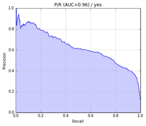
The merits of evaluating a model may be different for different tasks. As stated in Section 4.2, the data set selected by the experiment is unbalanced. The negative sample 0 value in the data set accounts for 88.7% of the total data set. If our model "predicts" all target variable values ​​to 0, then it is accurate. Accuracy should be around 88.7%. However, obviously, this "prediction" has no meaning. Therefore, we prefer to be able to predict a positive sample (y = 1) model. Therefore, in the experiment, the f1-score of the positive sample is used as a criterion for evaluating the pros and cons of the model (other similar evaluation indicators such as AUC can also be used). The code for training and evaluation is as follows:
Def train_evaluate(train_data, test_data, classifier, n=1, frac=1.0, threshold = 0.5):
Train_data = resample_train_data(train_data, n, frac)
train_X = train_data.drop('y', axis=1)
Train_y = train_data['y']
test_X = test_data.drop('y', axis=1)
Test_y = test_data['y']
Classifier = classifier.fit(train_X, train_y)
Prodict_prob_y = classifier.predict_proba(test_X)[:,1]
Report = classification_report(test_y, prodict_prob_y > threshold,
Target_names = ['no', 'yes'])
Prodict_y = (prodict_prob_y > threshold).astype(int)
Accuracy = np.mean(test_y.values ​​== prodict_y)
Print("Accuracy: {}".format(accuracy))
Print(report)
Fpr, tpr, thresholds = metrics.roc_curve(test_y, prodict_prob_y)
Precision, recall, thresholds = metrics.precision_recall_curve(test_y, prodict_prob_y)
Test_auc = metrics.auc(fpr, tpr)
Plot_pr(test_auc, precision, recall, "yes")
Return prodict_y
The training evaluation function can be used to select the model, select the logistic regression model and the random forest model respectively, and adjust the values ​​of the respective parameters separately, and finally select the random forest model with the highest f1-score. Specifically, when n_estimators is set to 400, 7 times oversampling is performed on the positive samples (n=7), negative samples are not negatively sampled (frac=1.0), and the positive sample classification threshold is 0.40 (threshold), that is, when When a probability that a sample belongs to a positive sample is greater than 0.4, the sample is classified as a positive sample.
Forest = RandomForestClassifier(n_estimators=400, oob_score=True) prodict_y = train_evaluate(train_data, test_data, forest, n=7, frac=1, threshold=0.40)
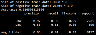
The evaluation results of this model on the cross-check set are as follows:
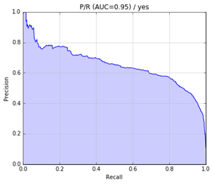
The precision-recall curve is as follows:
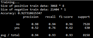
Finally, the model is applied to the test set, and the test results are as follows:
The precision-recall curve is as follows:
5. Outlook
You can also consider the following aspects to improve the F1 score:
More detailed feature selection, such as derived attributes;
Use better methods to solve data imbalance problems, such as cost-sensitive learning methods;
More detailed adjustments;
Try other classification models such as neural networks;
Single Voltage AC180-240V Led Driver
Single Voltage AC180-240V Led Driver
Quick Overview
Constant current mode output
Typical lifetime>50000 hours
Protections: Short circuit/ Over Voltage/ Over temperature
Parameter:
Input voltage: 100-130vac / 180-240vac
output voltage: 25-40vdc / 27-42vdc / 35-45vdc / 50-70vdc
current: 100mA-2000mA.
Power factor: >0.9
Dimming:Traic
>=50000hours, 3-5 years warranty.
certificate: UL CE FCC TUV SAA ect.


What's the benefits of Fahold Driver?
- Standard Linear Lighting
- Cost-effective led driver solution for industry,commercial and other applications
- Good quality of led driver with high efficiency output to meet different requirements
- Easy to order and install,requiring less time,reducing packaging waste and complexity
- Flexible solution
FAQ:
Question 1:Are you a factory or a trading company?
Answer: We are a factory.
Question 2: Payment term?
Answer: 30% TT deposit + 70% TT before shipment,50% TT deposit + 50% LC balance, Flexible payment
can be negotiated.
Question 3: What's the main business of Fahold?
Answer: Fahold focused on LED controllers and dimmers from 2010. We have 28 engineers who dedicated themselves to researching and developing LED controlling and dimming system.
Question 4: What Fahold will do if we have problems after receiving your products?
Answer: Our products have been strictly inspected before shipping. Once you receive the products you are not satisfied, please feel free to contact us in time, we will do our best to solve any of your problems with our good after-sale service.
Led Driving Lights Driver,60Watt Led Driver,Current Led Driver
ShenZhen Fahold Electronic Limited , https://www.fahold.net